Controlling the Astorino Robot on a sphere
In this article, you will learn:
- how to simulate the motion of the Astorino robot on the surface of a sphere using the astorinoIDE software,
- how to use the mathematical description of a sphere to generate points on its surface,
- how to create a Python program that automatically calculates the robot’s position and orientation on the sphere,
- how to implement motion control of the robot on the surface of a sphere in astorinoIDE.
Thanks to this guide, you will learn how to simulate the movement of the Astorino robot over the surface of a sphere using astorinoIDE, and then implement and test the control program in real-world conditions. We’ll start with the mathematical description of the robot’s motion trajectory, then create Python code that calculates the robot’s position and orientation on the sphere’s surface. Finally, we’ll transfer the program to astorinoIDE and test it on the Astorino educational robot, verifying the correctness of the movement.
Required Equipment and Software
- astorino robot with control software,
- astorinoIDE software,
- ASTORINO-OPT-SIMBOX (for simulation testing),
- Python development environment (with NumPy library),
- PC with Windows operating system.
Introduction
Controlling a robot in three-dimensional space is a challenge, especially when precise navigation on a spherical surface is required. Robots must handle complex trajectories that may involve motion along straight lines as well as more intricate surfaces such as a sphere.
This article presents two methods for controlling the Astorino robot to perform motion on a spherical surface. The first method involves shifting the Tool Center Point (TCP) to the center of the sphere, while the second method uses a mathematical description of the sphere along with appropriate coordinate system transformation. The following sections of the article detail how these methods are implemented in astorinoIDE and how to generate the robot’s trajectory.
Motion Control on a Sphere Based on the TCP Point
The first method of controlling motion on a sphere involves moving the TCP to the center of the sphere. To do this, the tool frame (TOOL) must be offset from the robot’s end-effector (tool or flange), and then the robot must be positioned in such a way that the TCP coincides with the center of the sphere. Once this position is achieved, rotating the robot around the X and Y axes of the TOOL frame results in motion along the sphere’s surface. This kind of control is relatively simple but may require precise initial configuration.
Control Based on the Mathematical Description of a Sphere
Parameters Used to Describe a Position on the Sphere’s Surface
An alternative approach to moving the robot on a sphere is to use its mathematical description in 3D space. This can be done by defining appropriate parameters of the sphere and computing the position and orientation of points on its surface. The following notations will be used:
- S(x0,y0,z0) – center of the sphere,
- P(x,y,z) – arbitrary point on the sphere’s surface,
- Rk– radius of the sphere,
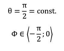
- θ – zenith angle
- Φ – azimuth
The zenith angle is the angle between the global vertical axis (Z axis) and the vector from the center of the sphere to a point on its surface. This angle is positive when measured from the Z axis in the direction of the radius leading to a given point on the sphere.
The azimuth is the angle between the X axis and the projection of the vector leading from the center of the sphere to a point on its surface onto the XY horizontal plane. This angle is positive when measured from the X axis toward the Y axis.
These angle definitions are illustrated below (Figure 1).
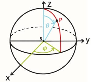
Fig. 1 Illustration showing the zenith angle and azimuth angle. Source: ASTOR
Example based on the earth as a sphere:
- zenith angle (θ) – defines the geographic latitude
- azimuth (φ) – defines the geographic longitude
Mathematical description of position and orientation on a sphere
Using the above angular definitions, the position on the surface of a sphere can be described by the following formulas:
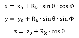
The tool’s orientation should be defined so that its Z-axis is perpendicular to the sphere’s surface and directed toward the center of the sphere.
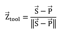
The Z-axis vector is defined as the normalized vector pointing toward the center of the sphere.
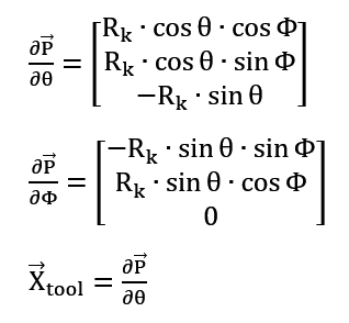
Next, it is necessary to determine the X-axis. It will be defined as tangent to the surface of the sphere, determined based on the derivative of the position with respect to the zenith angle. If the zenith angle is constant (resulting in a zero derivative), the X-axis will be defined as the derivative of the position with respect to the azimuth angle. The following formulas are used to calculate this orientation:
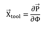
 However, if the derivative is close to zero, we take the direction of the X axis as:
In the final step, the direction of the X-axis should be recalculated to ensure the orthonormality of the tool’s coordinate system.
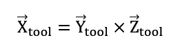
Given the vectors:
we can construct the rotation matrix:
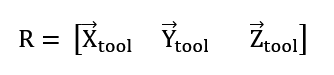
Based on it, we can determine the Euler angles (in the ZYZ convention), which uniquely describe the orientation of the tool in 3D space.
Implementation of control in the astorinoIDE program
First, launch the astorinoIDE program. Select the type of connection from the dropdown list (in this example, USB connection was chosen) and click the Connect/Disconnect button (Fig. 2).
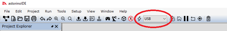
Fig. 2. View of the top toolbar in astorinoIDE. Source: ASTOR
Select the direction of data transfer from the computer to the robot and click SYNC (Fig. 3).
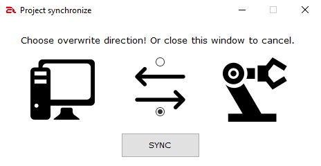
Fig. 3. View of the synchronization window for the connection between the computer and the robot. Source: ASTOR
Next, open or create a new project from the top toolbar. To do this, click Project and choose the appropriate option from the dropdown list (Fig. 4).
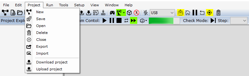
Fig. 4. View of the menu for creating or opening projects. Source: ASTOR
Then, open or create a new program. From the left folder tree, you can select an existing file from the Program Files tab or create a new program using the options in the top bar under the File tab. After choosing to create a new program (Fig. 5), a window will appear where you enter the file name and confirm with the OK button (Fig. 6).
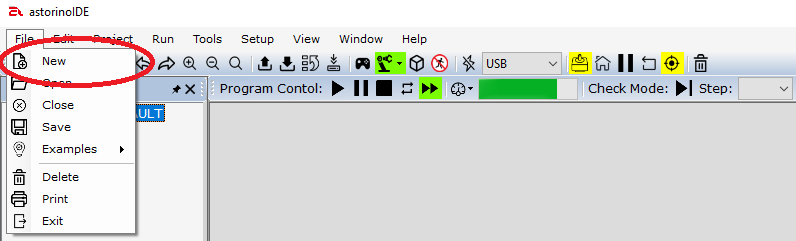
Fig. 5. View of the program editing menu. Source: ASTOR
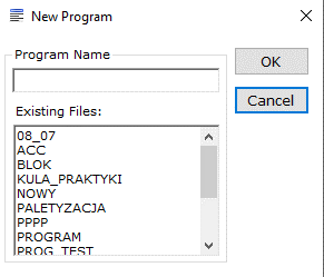
Fig. 6. View of the new program creation window. Source: ASTOR
After connecting to the robot and creating your own program, you can start building the scene (the robot setup with the sphere in space). To open the simulation, click the Visualization button (Fig. 7), marked on the main program toolbar with a cube symbol.
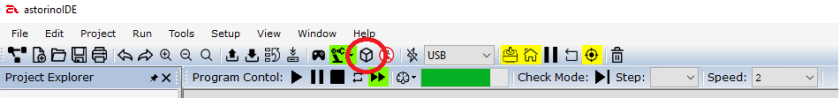
Fig. 7 View of the astorinoIDE top toolbar. Source: ASTOR
After clicking, a window with the robot should appear (Fig. 8).
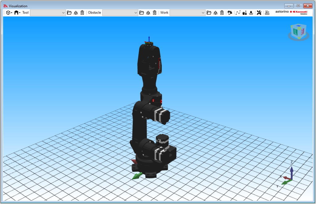
Fig. 8. View of the robot simulation window. Source: ASTOR
To facilitate robot control, we can bring it to the home position. This procedure allows for quickly returning the robot to its starting position, which simplifies further programming and command execution. To do this, in the terminal at the bottom of the astorinoIDE program (Fig. 9), type the command home and confirm by pressing Enter on the keyboard.
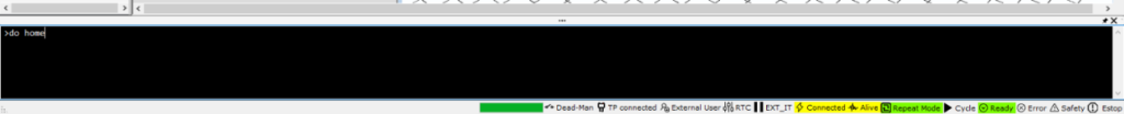
Fig. 9. View of the terminal window with the home command entered (click to enlarge). Source: ASTOR
After issuing this command, the terminal should respond with the message “DO motion Completed” (Fig. 10), and the robot should move to the home position (Fig. 11).

Fig. 10. View of the terminal window after executing the move to home position (click to enlarge). Source: ASTOR
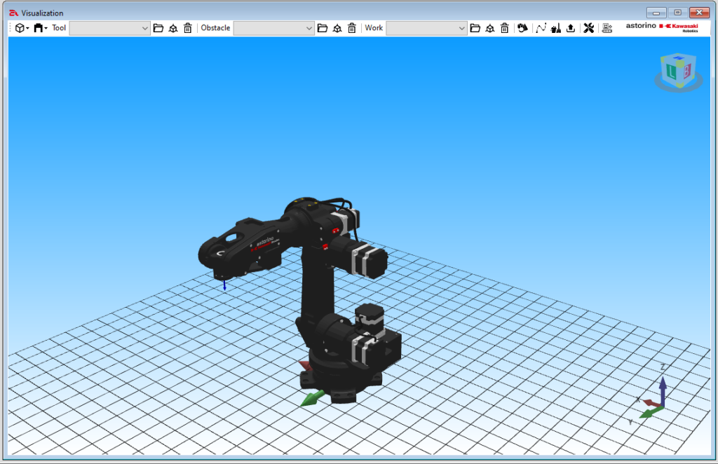
Fig. 11. View of the robot simulation window after moving to the home position. Source: ASTOR
NOTE! Remember that for the movement to be executed, the robot must be in Repeat Mode. You can change this in the top toolbar under: Mode -> Switch to Repeat (robot icon) (Fig. 12).
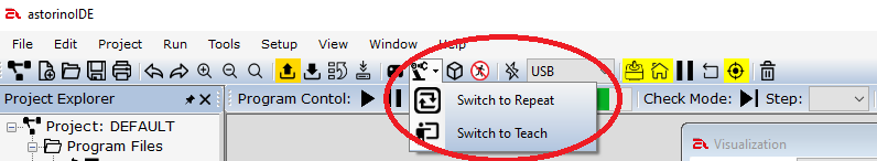
Fig. 12. View of the top toolbar in astorinoIDE when changing the movement mode. Source: ASTOR
Once the project with your program and the simulation window are open, you can add a sample sphere that the robot will later move around. To do this, in the visualization window select the option Open Shape Generator (Fig. 13).

Fig. 13. View of the top bar of the robot simulation window. Source: ASTOR
A shape creation window will open on the right side of the simulation. To add a sphere, select the Sphere tab (Fig. 14). Then you can enter its parameters: name, radius, position in the three global coordinate axes, color, and object type:
- Obstacle – these are static objects on the scene,
- Work – these objects can be moved by the robot,
- Tool – these objects always move along with the robot’s end effector.
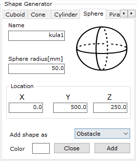
Fig. 14. View of the shape generator window in astorinoIDE. Source: ASTOR
After setting all parameters, click the Add button.
Moving on the Sphere by Rotating Around a Distant TCP Point
The first method of moving on the sphere is to move the TCP point away by a distance equal to the sphere’s radius. To do this, open the Robot Manager window (Fig. 15).
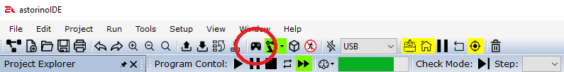
Fig. 15. View of the top toolbar in astorinoIDE. Source: ASTOR
Once the window appears, go to the TOOL tab on the right side (Fig. 16) and enter the previously set sphere radius value for the TOOL Z parameter.
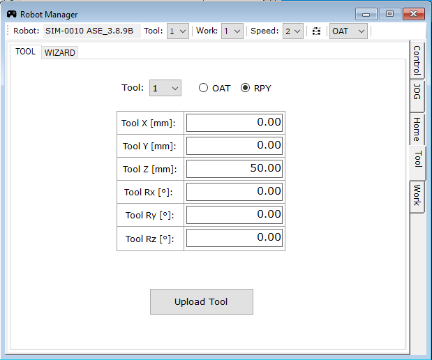
Fig. 16. View of the TOOL tab in the Robot Manager window. Source: ASTOR
Click Upload Tool and confirm the tool change after the warning appears.
Next, move the robot so that the TCP point coincides with the center of the sphere and the tool orientation is perpendicular to the sphere’s surface. You can use the JOG tab in the Robot Manager window to do this (Fig. 17). Choose the coordinate system you want to use to move the robot from the dropdown list (Jogging -> Mode), and use the buttons to move it to the position mentioned earlier (Fig. 18). This is possible only after switching the mode to Teach Mode.
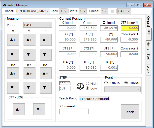
Fig. 17. View of the JOG tab in the Robot Manager window. Source: ASTOR
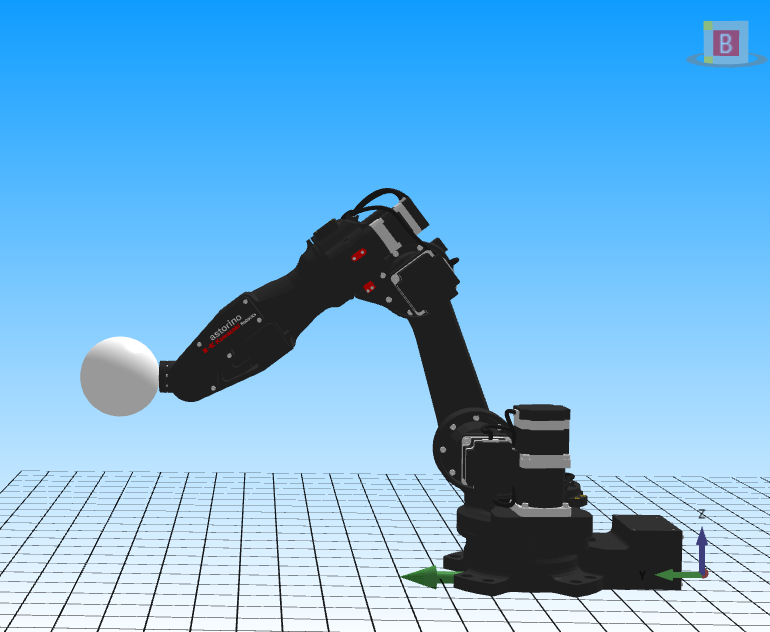
Fig. 18. View of the robot simulation after moving to the sphere’s surface. Source: ASTOR
Then you can move the robot along the sphere. To do this, in the JOG tab, select movement in the TOOL coordinate system and perform rotations around the X and Y axes (rotation around the Z axis is not meaningful here, since it was previously aligned perpendicular to the sphere’s surface). Below are some example robot positions.
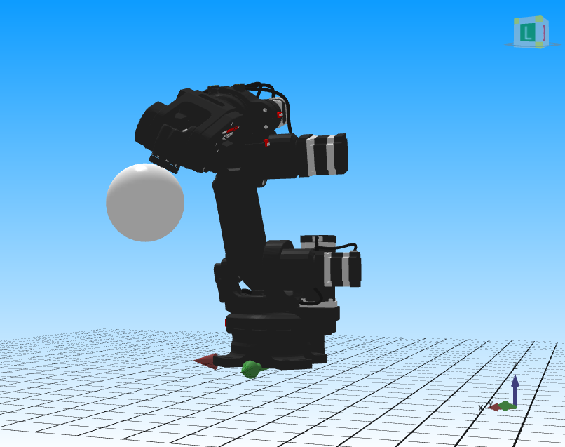
Fig. 19. Example robot position no. 1. Source: ASTOR
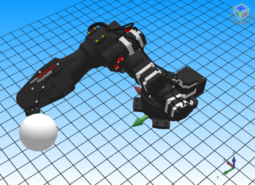
Fig. 20. Example robot position no. 2. Source: ASTOR
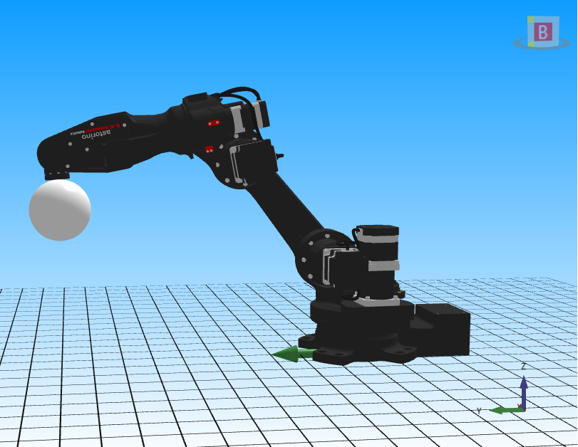
Fig. 21. Example robot position no. 3. Source: ASTOR
Movement on the sphere using Its mathematical description
The second method for moving the robot along the sphere is generating points (position and orientation) based on the description provided earlier in the article. A Python program was written for this purpose, which generates points on the surface of the sphere along with the orientation of the TOOL coordinate system.
Note! If the position or orientation of the TOOL coordinate system has been changed, as in the previous section, it should be reset to the default settings (by zeroing each position and orientation component – Fig. 22).
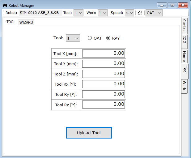
Fig. 22. View of the Tool tab in the Robot Manager window. Source: ASTOR
The versatility of the developed code allows calculating the position and orientation of the tool coordinate system in spherical space, regardless of the sphere’s position or radius. This enables calculating coordinates of points on the sphere’s surface in various configurations.
However, it should be noted that the program does not consider the actual robot constraints, such as its physical movement capabilities, reach, or tilts. In practice, this means the points provided by the program may not always be reachable by the robot under real conditions. The program only provides mathematical results referring to an ideal mathematical sphere model, without considering physical limitations of the robot, such as kinematics, reach, or mechanical constraints.
Thus, there is a need for further verification of the results in the context of real robot trajectories for specific applications. This article focuses on the implementation of the motion itself, not on specific applications.
To simplify the code and avoid overly complex names, the following notations were used:
- Zenith angle: θ = u
- Azimuth: Φ = v
Below is the Python code that generates a selected number of points on the surface of a sphere with any previously chosen parameters:
import numpy as np
from scipy.spatial.transform import Rotation as R
#Sphere parameters
x0, y0, z0 = 0.0, 500.0, 250.0 # center of the sphere
R_sphere = 50.0 # radius
N = 20 # number of points
for i in range(N):
u = i * np.pi / (N – 1) # zenith angle
v = np.pi # azimuth
#Position on the sphere surface
x = x0 + R_sphere * np.sin(u) * np.cos(v)
y = y0 + R_sphere * np.sin(u) * np.sin(v)
z = z0 + R_sphere * np.cos(u)
position = np.array([x, y, z])
center = np.array([x0, y0, z0])
#TOOL Z axis (towards sphere center)
Z_tool = center – position
Z_tool /= np.linalg.norm(Z_tool)
#Two tangent vectors to the surface (derivatives w.r.t u and v)
dP_du = np.array([
R_sphere * np.cos(u) * np.cos(v),
R_sphere * np.cos(u) * np.sin(v),
-R_sphere * np.sin(u)
])
dP_dv = np.array([
-R_sphere * np.sin(u) * np.sin(v),
R_sphere * np.sin(u) * np.cos(v),
0.0
])
#Choose one tangent vector (e.g., dP_dv)
tangent = dP_dv
if np.linalg.norm(tangent) < 1e-6: # safeguard against zero vector
tangent = dP_du
tangent /= np.linalg.norm(tangent)
#Build coordinate system
X_tool = tangent
Y_tool = np.cross(Z_tool, X_tool)
Y_tool /= np.linalg.norm(Y_tool)
X_tool = np.cross(Y_tool, Z_tool)
X_tool /= np.linalg.norm(X_tool)
#Rotation matrix and conversion to Euler angles
R_matrix = np.column_stack((X_tool, Y_tool, Z_tool))
rot = R.from_matrix(R_matrix)
euler_deg = rot.as_euler(‘zyz’, degrees=True)
#Output format: x,y,z,roll,pitch,yaw
print(f”{x:.3f},{y:.3f},{z:.3f},{euler_deg[2]:.3f},{euler_deg[1]:.3f},{euler_deg[0]:.3f}”)
The program calculates positions and orientations of a set of points located on the sphere surface. Initially, it defines basic parameters of the sphere: its center in 3D space, radius, and the number of points to be distributed on the surface.
Then, in a loop, it calculates the exact position of each point on the sphere, changing only the zenith angle while keeping the azimuth constant. This way, the points are distributed along one meridian. For each point on the sphere, a vector is calculated pointing from the point towards the sphere’s center. This vector determines the direction the tool or the local coordinate system “looks” at — this is the Z axis of the local frame.
To define full orientation in space, the X and Y axes are also needed. For this, two tangent vectors to the sphere surface are computed as derivatives of the point’s position with respect to the spherical angles. One of these tangent vectors is selected as the base for the X axis; if its length is too small, the other vector is chosen. The selected vector is normalized to length 1.
Next, an orthogonal coordinate system is constructed. The Y axis is determined as perpendicular to both the Z axis and the chosen tangent vector, and then the X axis is recalculated to ensure the three axes form a consistent right-handed coordinate system. These three vectors create a rotation matrix describing how the local coordinate system at the point is oriented relative to the global system. Finally, Euler angles are extracted from this matrix, describing the orientation as a sequence of rotations around axes. The position and these three angles are printed out, providing complete spatial information.
To verify the correctness of the generated points, a simple program was developed in astorinoIDE that uses three of the previously calculated points on the sphere surface. The program performs the robot’s movement along an arc, where the first point is the start point, the second is an auxiliary point, and the third is the endpoint. This method allows visually checking if the robot correctly follows the designated trajectory. Below is the code for the program executing this movement:
.PROGRAM SPHERE
HOME
lappro P1, 100
lmove P1
c1move P2
c2move P3
ldepart 100
.END
To transfer the calculated points into astorinoIDE, it is enough to copy the desired points returned by the Python program’s output. After generating the points, they must be manually entered into the robot environment, allowing further use in subsequent application stages. Below is an example of output after compiling the Python code (Fig. 23).
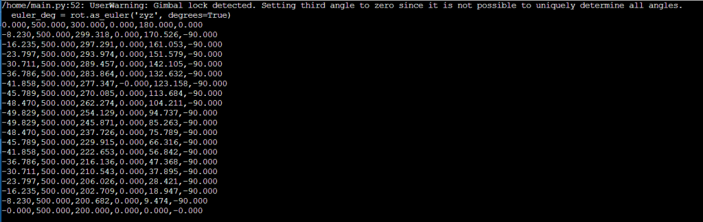
Fig. 23. Sample output from the Python program compilation for the example parameters (click to enlarge). Source: ASTOR
Note the warning indicating the detection of a “gimbal lock” during the conversion of rotation to Euler angles in the ‘zyz’ system. This means one rotation axis coincides with another, making one angle (the third) ambiguous and therefore set to zero.
If you want to transfer the first point to astorinoIDE, use the POINT and TRANS commands in the terminal (Fig. 24).

Fig. 24. Terminal window with instruction to create a new point (click to enlarge). Source: ASTOR
After confirming with Enter, the point will be saved. To check if this indeed happened, go to the Points -> Transformation tab. A window will display saved points (Fig. 25), where you should see your saved point as below:
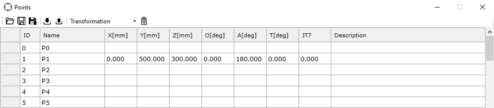
Fig. 25. Cartesian points window in astorinoIDE. Source: ASTOR
Repeat this process for the other two points. It is important that each point is declared under a different index, e.g., p2, p3, etc., to maintain consistency in the program and enable proper assignment to spatial positions of the robot.
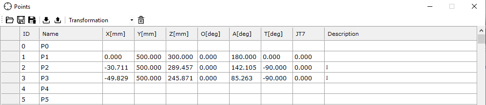
Fig. 26. Cartesian points window in astorinoIDE. Source: ASTOR
To test the program, start the cycle by clicking the Cycle Start button.
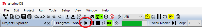
Fig. 27. Top toolbar view in astorinoIDE. Source: ASTOR
If you want to run the program from the beginning or from a specific step (not the first one), press Pause then Cycle Stop. Then select the code line from the Step dropdown menu where you want to start execution. Start the movement by clicking Pause, then Cycle Start.
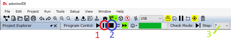
Fig. 28. Top toolbar view in astorinoIDE. Source: ASTOR
The program result is shown in the figure below:
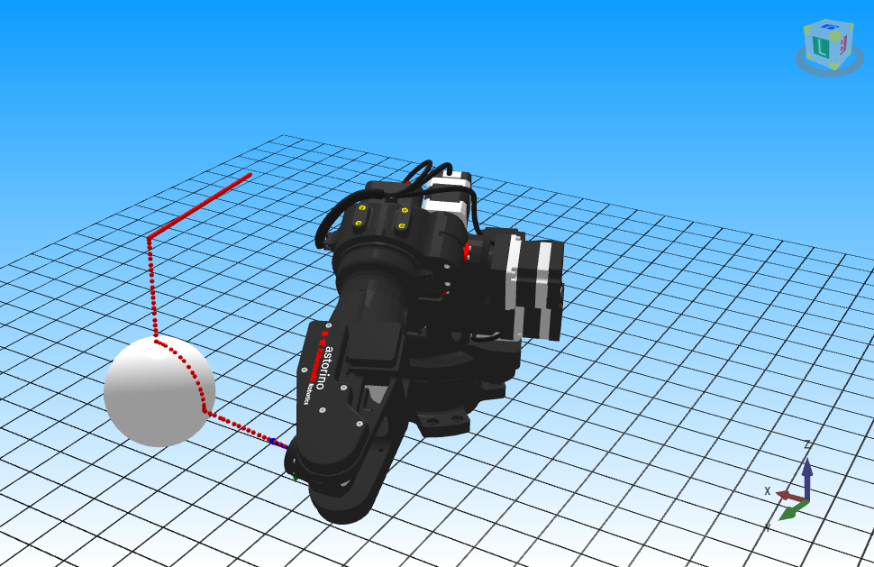
Fig. 29. Example program running a movement on the sphere with trajectory no. 1 highlighted. Source: ASTOR
Analysis shows the azimuth value remains constant (Fig. 29), while the zenith angle changes from 0 to about 90, with the last point characterized by this angle. The movement occurs only in the XZ plane (for y = const. = y0).
The program was also tested for other zenith and azimuth angle values. This time the following zenith θ and azimuth Φ values were used:
The azimuth value changes in the loop according to the formula:
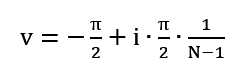
The corresponding Python code line is:
v = -np.pi / 2 + i * (np.pi / 2) / (N – 1))
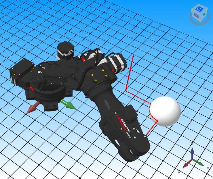
Fig. 30. Example program running movement on the sphere with trajectory no. 2 highlighted. Source: ASTOR
In this case (Fig. 30), the zenith angle remains constant, causing movement in the XY plane (for z = const. = z0).
Below are two other generated trajectories:
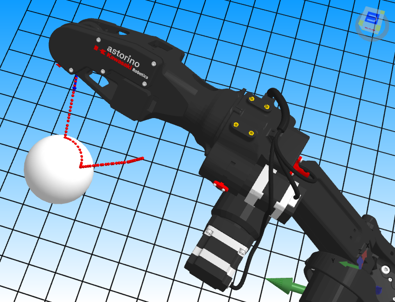
Fig. 31. Example program running movement on the sphere with trajectory no. 3 highlighted. Source: ASTOR
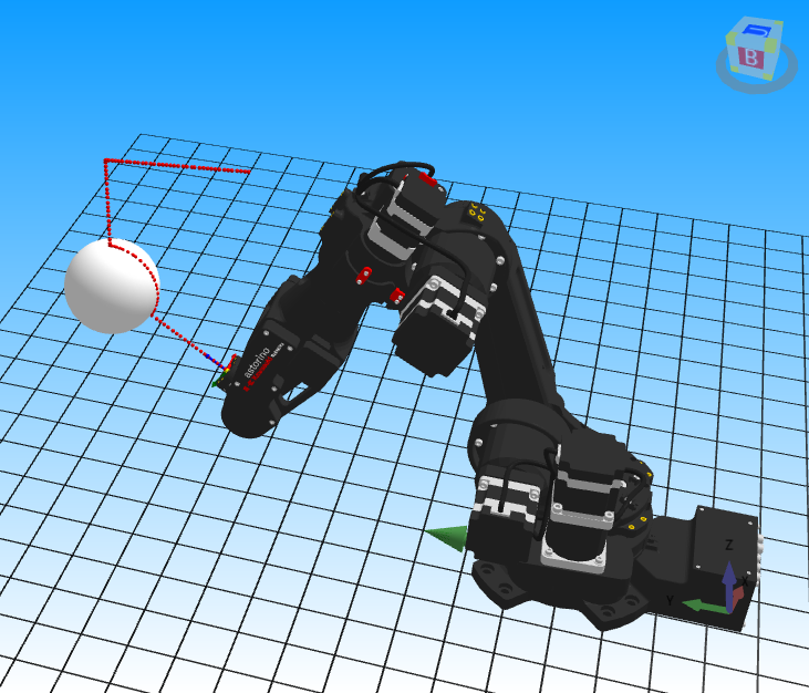
Fig. 32. Example program running movement on the sphere with trajectory no. 4 highlighted. Source: ASTOR
This article presented two methods for controlling the Astorino robot over a sphere’s surface, each with advantages and limitations. The first method is simpler and more intuitive, based on straightforward geometric calculations. The second method, although more complex, allows for greater flexibility and precision, as it enables the generation of points and tool orientation based on the mathematical description of a sphere.
The practical implementation of control in the astorinoIDE software allows for the simulation of the robot’s movements, which is essential for testing the correctness of trajectories before they are executed in the real world. Both the control methods and the implementation in astorinoIDE provide a solid foundation for the further development of Astorino robot control technology on spherical surfaces. In the future, they can be adapted for more advanced applications that require precise motion along more complex trajectories or even within spaces of more intricate shapes.