Object Detection ‘On the Fly’ with Kawasaki Robotics – Comparison of HSENSE and XMOVE Functions
In this article, you will learn:
- how to perform precise positioning in handling applications,
- what the HSENSE and XMOVE functions are and how they work,
- how to use these functions for accurate positioning.
In simplified terms, a robot working in a general handling application is typically tasked with moving an object from point A to point B. When all elements are perfectly aligned and in place, this task is straightforward to perform and quick to program. However, as we know, it is extremely rare for everything to be perfectly positioned. For the system to operate efficiently, the elements need to be either positioned accurately or located dynamically. So how do we deal with situations where the dimensions and position of the object may vary from the expected values?
In such cases, we need to equip the robot with a sense of vision or touch to locate and measure the target object. This can be done using 2D or 3D vision systems, which, however, may prove too expensive to achieve a reasonable ROI – especially considering that only a small fraction of their capabilities may be used in the application.
For basic object detection, simple sensors are often sufficient – such as optical, capacitive, inductive, or others – depending on the material and the required type of detection. However, these sensors typically only provide information about the presence of the object. So how can we actually measure and orient the object in space?
By combining object detection data, the robot’s position, mathematics, and a bit of engineering ingenuity, we can determine and recognize many geometric features of the object as well as its position relative to the robot.
Definition of the Engineering Problem
Let us now follow the below engineering problem:
At the pick-up station, there are steel discs with known diameter and thickness. They are manually placed into a pick up socket. The stack always contains 3 pieces, and once all are used, it is refilled by the operator. The parts are picked up by a jaw gripper. The robot is equipped with an optical sensor. The sensor spot has a diameter of 2 mm. Our gripper has a clearance of 7 mm between the jaws and the object when the jaws are fully open. A positional error greater than 7 mm will result in a robot collision. How can we find the centers of the circles (discs), which will serve as pick-up positions?
Calculations
To determine the center of a circle, we need at least 3 points located on its circumference.
Equation for a Circle in a Plane
For a circle lying on a 2D plane, the calculations are as follows:
1. Plane equations:
![]()
2. Substitute the coordinates of 3 points into the equation:
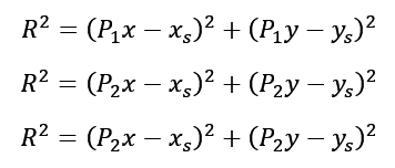
3. Form a system of equations based on these formulas:
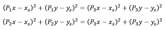
Then, using formulas of squared binomials, we transform the system of equations to obtain values for xs and ys, which denote the center of the desired circle.
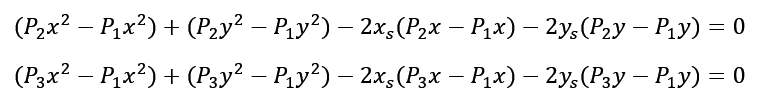
By applying the substitution method

we can find the coordinates xs and ys:
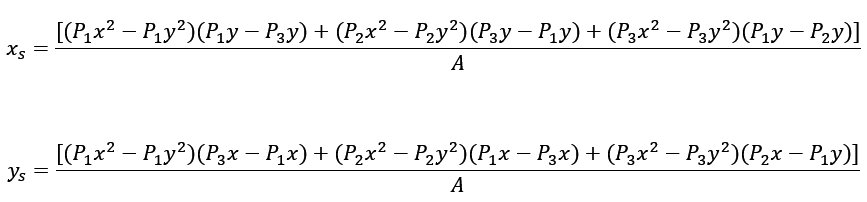
By substituting the known coordinates of the points on the circle into the above formulas, we obtain the coordinates of the circle center.
Equations for 3D Space
The above derivation is a simplification because the robot operates in 3D space. To stay focused on the core topic of this article, the derivation for the 3D case is presented in an appendix at the end of the article.
Recording the calculation in the robot program
The 2D plane point calculations are already quite complex and time-consuming to manually implement as mathematical functions in a robot program. Fortunately, we don’t need to write them ourselves, as a ready-made function exists for finding the circle center: CCENTER.
CCENTER(pose1, pose2, pose3, pose4)
Points 1–3 must lie on the circle, and the fourth point serves to copy the desired orientation.
Engineering problem software
Mathematical part complete. How do we now find 3 points on the edge of our object?
Typically, programmers use the XMOVE function, which allows the robot to move until a specified input signal is detected. The robot then stops, and after stopping, the programmer records the current TCP position as the detection point. The downside of this approach is that the sensor signal must remain stable for at least 50 ms to be recognized as a detection. Additionally, the robot’s deceleration path must be considered. If a robot with a heavy gripper is braking from high speed, it may slightly miss the actual detection position.
When using the program shown below, the detection point will depend on the sensor response time, its hysteresis, and the TCP speed of the robot. The higher the speed, the further away the point detect1 will be from the actual detected edge.
XMOVE pt1 TILL 1001
BREAK
HERE detect1
…
The function that records the robot’s position to memory at the exact moment the sensor detects an object is called HSENSE. It monitors the sensor signal status and, when a change is detected, saves the current joint position to a buffer. Unlike XMOVE, HSENSE does not require the robot to stop its motion, and the required signal duration is much shorter. Typically, 2 ms is enough, as this corresponds to the input refresh rate for most Kawasaki controllers.
How can we practically use the functions described above?
Example program using XMOVE
TOOL sensor_tool ; setting the sensor as TCP
;———————————————————–
; Move to the search position
;———————————————————–
HOME
LMOVE start
;———————————————————–
; Move through the expected positions of the stack
;———————————————————–
ACCURACY 1 FINE
SPEED search_speed mm/s
XMOVE p1 TILL 1001
BREAK
HERE found1
SPEED search_speed mm/s
LMOVE p1
SPEED search_speed mm/s
XMOVE p2 TILL 1001
BREAK
HERE found2
SPEED search_speed mm/s
LMOVE p2
SPEED search_speed mm/s
XMOVE p3 TILL 1001
BREAK
HERE found3
SPEED search_speed mm/s
LMOVE p3
MVWAIT 1
LDEPART 100
;———————————————————–
; Calculate the center position of the circle
;———————————————————–
POINT cylinder_x = CCENTER(found1, found2, found3, start)
Example program using HSENSE
TOOL sensor_tool ; setting the sensor as TCP
;———————————————————–
; Move to the search position
;———————————————————–
SPEED 500 mm/s
LMOVE start
;———————————————————–
; Activate HSENSE function parameters
;———————————————————–
HSENSESET 1 = 1001, 20
;———————————————————–
; Pass through the expected stack positions
;———————————————————–
ACCURACY 1 FINE
SPEED search_speed mm/s ALWAYS
LMOVE p1
LMOVE p2
LMOVE p3
MVWAIT 1
;
.num = 0
loop:
HSENSE1 .result_var, sig_status[.num+1], #hsense_pos[.num+1], .err_var, .mem
IF .err_var <> 0 THEN
.err = 3
RETURN
END
;
IF .result_var == TRUE AND sig_status[.num+1] == TRUE THEN
POINT detect[.num+1] = #hsense_pos[.num+1]
.num = .num + 1
END
IF .mem GOTO loop
;
HSENSESET 1 = 0
SPEED 500 mm/s
LDEPART 100
;———————————————————–
; Calculate the center position of the circle
;———————————————————–
POINT cylinder = CCENTER(detect[1], detect[2], detect[3], start)
Comparison of Results
The key parameters for comparing both solutions are: program execution time and detection accuracy. In most robotic applications, we focus on two factors: precision and performance. When we have access to high-end equipment, such as Kawasaki Robotics robots, it’s worth leveraging their full potential through smart programming and optimized code. Sampling speeds for search movements were assumed as shown in the table below. All other movements are performed at a speed of 500 mm/s.

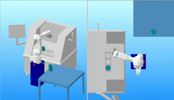
Comparison of Achieved Accuracy Relative to the Position in K-Roset:
The center of the workpiece in K-Roset was set at position X = 300, Y = 600 relative to the robot’s base coordinate system.
By using a simple distance formula between a point and the center of the circle, we can determine whether the robot is able to safely pick up the part without collision.
Green indicates test results that met our assumptions for collision free operation.
Summary
As demonstrated by the tests, the HSENSE function performs very well in non-contact measurement applications. A buffer of 20 detection positions, the ability to react to both rising and falling signal edges, and the possibility of simultaneously monitoring two signals provide a wide range of capabilities. In object detection scenarios where there is no collision risk, HSENSE can significantly reduce search time, and therefore also improve the overall cycle time of the application.
The XMOVE function performs well when detecting objects at low speeds. It can be used for measurements, but it is primarily designed for detecting objects along the robot’s motion path, so that the detected object can be picked up in the next step.
As the test results have shown, both functions can be used for object detection. However, to fully utilize their potential, they should be applied where each shows its clear advantage.
The HSENSE function works well for noncontact measurements where we can quickly determine points on the edges of an object. However, it is not suitable when the object detection happens along a collision path.
XMOVE shows its advantage in detecting and picking up a part located directly on a collision path. By using two sensors and cascading the XMOVE functions, we can approach, for example, a stack of separators at high speed. After detection at a safe distance by the first sensor, we reduce the robot TCP speed and then search for the exact height of the separator on the stack at a low speed. Once detected, we stop the robot and pick up the separator, all on a single motion path.
Using the right combination of these two functions allows us to unlock the full potential of both efficiency and precision in our robotic application.
Appendix
Derivation of formulas for a circle in three-dimensional space
Let’s assume points:
![]()
which lie on the circle. The center of the circle at point S has the following coordinates:
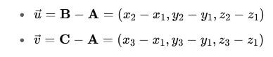
1. Calculate vectors between points A, B, C:
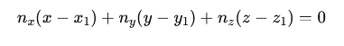
2. Determine the equation of the plane:
![]()
3. Knowing that the points on the circle are equally distant from the center of the circle by the radius:
![]()
Simplifying the formula, we get:

Similarly, for points A and C, we can write an equation:

The third equation comes from the fact that point O lies on the plane defined by points A, B, and C:
4. We set up and solve a system of three linear equations, using the substitution method to simplify the notation.
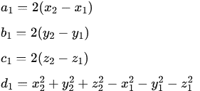
For the first equation, we assume:
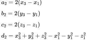
Similarly, for the second equation:
And for the third equation:
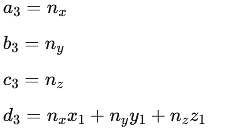
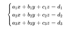
We obtain the following system of equations:
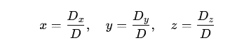
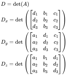
5. Using Cramer’s rule, we write the system in matrix form and calculate the determinants of the matrices:
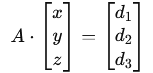
The main matrix A has the following form:
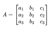
Finally, we calculate the determinants of the matrices:
6. After transformations, we obtain the coordinates of the center of the circle: